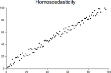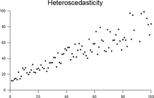

In statistics, a sequence of random variables is homoscedastic (/ˌhoʊmoʊskəˈdæstɪk/) if all its random variables have the same finite variance; this is also known as homogeneity of variance. The complementary notion is called heteroscedasticity, also known as heterogeneity of variance. The spellings homoskedasticity and heteroskedasticity are also frequently used. “Skedasticity” comes from the Ancient Greek word “skedánnymi”, meaning “to scatter”.[1][2][3] Assuming a variable is homoscedastic when in reality it is heteroscedastic (/ˌhɛtəroʊskəˈdæstɪk/) results in unbiased but inefficient point estimates and in biased estimates of standard errors, and may result in overestimating the goodness of fit as measured by the Pearson coefficient.
The existence of heteroscedasticity is a major concern in regression analysis and the analysis of variance, as it invalidates statistical tests of significance that assume that the modelling errors all have the same variance. While the ordinary least squares estimator is still unbiased in the presence of heteroscedasticity, it is inefficient and inference based on the assumption of homoskedasticity is misleading. In that case, generalized least squares (GLS) was frequently used in the past.[4][5] Nowadays, standard practice in econometrics is to include Heteroskedasticity-consistent standard errors instead of using GLS, as GLS can exhibit strong bias in small samples if the actual skedastic function is unknown.[6]
Because heteroscedasticity concerns expectations of the second moment of the errors, its presence is referred to as misspecification of the second order.[7]
The econometrician Robert Engle was awarded the 2003 Nobel Memorial Prize for Economics for his studies on regression analysis in the presence of heteroscedasticity, which led to his formulation of the autoregressive conditional heteroscedasticity (ARCH) modeling technique.[8]
- ^ For the Greek etymology of the term, see McCulloch, J. Huston (1985). "On Heteros*edasticity". Econometrica. 53 (2): 483. JSTOR 1911250.
- ^ White, Halbert (1980). "A heteroskedasticity-consistent covariance matrix estimator and a direct test for heteroskedasticity". Econometrica. 48 (4): 817–838. CiteSeerX 10.1.1.11.7646. doi:10.2307/1912934. JSTOR 1912934.
- ^ Gujarati, D. N.; Porter, D. C. (2009). Basic Econometrics (Fifth ed.). Boston: McGraw-Hill Irwin. p. 400. ISBN 9780073375779.
- ^ Goldberger, Arthur S. (1964). Econometric Theory. New York: John Wiley & Sons. pp. 238–243. ISBN 9780471311010.
- ^ Johnston, J. (1972). Econometric Methods. New York: McGraw-Hill. pp. 214–221.
- ^ Angrist, Joshua D.; Pischke, Jörn-Steffen (2009-12-31). Mostly Harmless Econometrics: An Empiricist's Companion. Princeton University Press. doi:10.1515/9781400829828. ISBN 978-1-4008-2982-8.
- ^ Long, J. Scott; Trivedi, Pravin K. (1993). "Some Specification Tests for the Linear Regression Model". In Bollen, Kenneth A.; Long, J. Scott (eds.). Testing Structural Equation Models. London: Sage. pp. 66–110. ISBN 978-0-8039-4506-7.
- ^ Engle, Robert F. (July 1982). "Autoregressive Conditional Heteroscedasticity with Estimates of the Variance of United Kingdom Inflation". Econometrica. 50 (4): 987–1007. doi:10.2307/1912773. ISSN 0012-9682. JSTOR 1912773.