Stable distribution

Stable

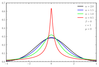
Probability density function Symmetric ${\displaystyle \alpha }$-stable distributions with unit scale factor Skewed centered stable distributions with unit scale factor
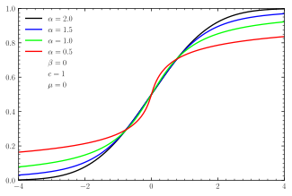
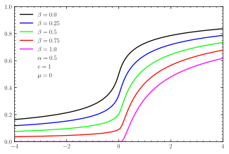
Cumulative distribution function CDFs for symmetric ${\displaystyle \alpha }$-stable distributions CDFs for skewed centered stable distributions
Parameters	${\displaystyle \alpha \in (0,2]}$ — stability parameter ${\displaystyle \beta }$ ∈ [−1, 1] — skewness parameter (note that skewness is undefined) c ∈ (0, ∞) — scale parameter μ ∈ (−∞, ∞) — location parameter
Support	x ∈ [μ, +∞) if ${\displaystyle \alpha <1}$ and ${\displaystyle \beta =1}$ x ∈ (-∞, μ] if ${\displaystyle \alpha <1}$ and ${\displaystyle \beta =-1}$ x ∈ R otherwise
PDF	not analytically expressible, except for some parameter values
CDF	not analytically expressible, except for certain parameter values
Mean	μ when ${\displaystyle \alpha >1}$, otherwise undefined
Median	μ when ${\displaystyle \beta =0}$, otherwise not analytically expressible
Mode	μ when ${\displaystyle \beta =0}$, otherwise not analytically expressible
Variance	2c2 when ${\displaystyle \alpha =2}$, otherwise infinite
Skewness	0 when ${\displaystyle \alpha =2}$, otherwise undefined
Excess kurtosis	0 when ${\displaystyle \alpha =2}$, otherwise undefined
Entropy	not analytically expressible, except for certain parameter values
MGF	${\displaystyle \exp \!{\big (}t\mu +c^{2}t^{2}{\big )}}$ when ${\displaystyle \alpha =2}$, ${\displaystyle \exp \!{\big (}t\mu -c^{\alpha }t^{\alpha }\sec(\pi \alpha /2){\big )}}$ when ${\displaystyle \alpha \neq 1,\beta =-1,t>0}$, ${\displaystyle \exp \!{\big (}t\mu -c2\pi ^{-1}t\ln t{\big )}}$ when ${\displaystyle \alpha =1,\beta =-1,t>0}$, otherwise undefined
CF	${\displaystyle \exp \!{\Big [}\;it\mu -|c\,t|^{\alpha }\,(1-i\beta \operatorname {sgn}(t)\Phi )\;{\Big ]},}$ where ${\displaystyle \Phi ={\begin{cases}\tan {\tfrac {\pi \alpha }{2}}&{\text{if }}\alpha \neq 1\\-{\tfrac {2}{\pi }}\log |t|&{\text{if }}\alpha =1\end{cases}}}$

In probability theory, a distribution is said to be stable if a linear combination of two independent random variables with this distribution has the same distribution, up to location and scale parameters. A random variable is said to be stable if its distribution is stable. The stable distribution family is also sometimes referred to as the Lévy alpha-stable distribution, after Paul Lévy, the first mathematician to have studied it.^[1][2]

Of the four parameters defining the family, most attention has been focused on the stability parameter, ${\displaystyle \alpha }$ (see panel). Stable distributions have ${\displaystyle 0<\alpha \leq 2}$, with the upper bound corresponding to the normal distribution, and ${\displaystyle \alpha =1}$ to the Cauchy distribution. The distributions have undefined variance for ${\displaystyle \alpha <2}$, and undefined mean for ${\displaystyle \alpha \leq 1}$. The importance of stable probability distributions is that they are "attractors" for properly normed sums of independent and identically distributed (iid) random variables. The normal distribution defines a family of stable distributions. By the classical central limit theorem the properly normed sum of a set of random variables, each with finite variance, will tend toward a normal distribution as the number of variables increases. Without the finite variance assumption, the limit may be a stable distribution that is not normal. Mandelbrot referred to such distributions as "stable Paretian distributions",^[3][4][5] after Vilfredo Pareto. In particular, he referred to those maximally skewed in the positive direction with ${\displaystyle 1<\alpha <2}$ as "Pareto–Lévy distributions",^[1] which he regarded as better descriptions of stock and commodity prices than normal distributions.^[6]