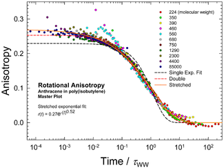
The stretched exponential function is obtained by inserting a fractional power law into the exponential function. In most applications, it is meaningful only for arguments t between 0 and +∞. With β = 1, the usual exponential function is recovered. With a stretching exponent β between 0 and 1, the graph of log f versus t is characteristically stretched, hence the name of the function. The compressed exponential function (with β > 1) has less practical importance, with the notable exception of β = 2, which gives the normal distribution.
In mathematics, the stretched exponential is also known as the complementary cumulative Weibull distribution. The stretched exponential is also the characteristic function, basically the Fourier transform, of the Lévy symmetric alpha-stable distribution.
In physics, the stretched exponential function is often used as a phenomenological description of relaxation in disordered systems. It was first introduced by Rudolf Kohlrausch in 1854 to describe the discharge of a capacitor;[1] thus it is also known as the Kohlrausch function. In 1970, G. Williams and D.C. Watts used the Fourier transform of the stretched exponential to describe dielectric spectra of polymers;[2] in this context, the stretched exponential or its Fourier transform are also called the Kohlrausch–Williams–Watts (KWW) function. The Kohlrausch–Williams–Watts (KWW) function corresponds to the time domain charge response of the main dielectric models, such as the Cole–Cole equation, the Cole–Davidson equation, and the Havriliak–Negami relaxation, for small time arguments.[3]
In phenomenological applications, it is often not clear whether the stretched exponential function should be used to describe the differential or the integral distribution function—or neither. In each case, one gets the same asymptotic decay, but a different power law prefactor, which makes fits more ambiguous than for simple exponentials. In a few cases,[4][5][6][7] it can be shown that the asymptotic decay is a stretched exponential, but the prefactor is usually an unrelated power.
- ^ Kohlrausch, R. (1854). "Theorie des elektrischen Rückstandes in der Leidner Flasche". Annalen der Physik und Chemie. 91 (1): 56–82, 179–213. Bibcode:1854AnP...167...56K. doi:10.1002/andp.18541670103..
- ^ Williams, G. & Watts, D. C. (1970). "Non-Symmetrical Dielectric Relaxation Behavior Arising from a Simple Empirical Decay Function". Transactions of the Faraday Society. 66: 80–85. doi:10.1039/tf9706600080. S2CID 95007734..
- ^ Holm, Sverre (2020). "Time domain characterization of the Cole-Cole dielectric model". Journal of Electrical Bioimpedance. 11 (1): 101–105. doi:10.2478/joeb-2020-0015. PMC 7851980. PMID 33584910.
- ^ Donsker, M. D. & Varadhan, S. R. S. (1975). "Asymptotic evaluation of certain Markov process expectations for large time". Comm. Pure Appl. Math. 28: 1–47. doi:10.1002/cpa.3160280102.
- ^ Takano, H. and Nakanishi, H. and Miyashita, S. (1988). "Stretched exponential decay of the spin-correlation function in the kinetic Ising model below the critical temperature". Phys. Rev. B. 37 (7): 3716–3719. Bibcode:1988PhRvB..37.3716T. doi:10.1103/PhysRevB.37.3716. PMID 9944981.
{{cite journal}}: CS1 maint: multiple names: authors list (link) - ^ Shore, John E. and Zwanzig, Robert (1975). "Dielectric relaxation and dynamic susceptibility of a one-dimensional model for perpendicular-dipole polymers". The Journal of Chemical Physics. 63 (12): 5445–5458. Bibcode:1975JChPh..63.5445S. doi:10.1063/1.431279.
{{cite journal}}: CS1 maint: multiple names: authors list (link) - ^ Brey, J. J. and Prados, A. (1993). "Stretched exponential decay at intermediate times in the one-dimensional Ising model at low temperatures". Physica A. 197 (4): 569–582. Bibcode:1993PhyA..197..569B. doi:10.1016/0378-4371(93)90015-V.
{{cite journal}}: CS1 maint: multiple names: authors list (link)
