
Structural equation modeling (SEM) is a diverse set of methods used by scientists for both observational and experimental research. SEM is used mostly in the social and behavioral science fields, but it is also used in epidemiology,[2] business,[3] and other fields. A common definition of SEM is, "...a class of methodologies that seeks to represent hypotheses about the means, variances, and covariances of observed data in terms of a smaller number of 'structural' parameters defined by a hypothesized underlying conceptual or theoretical model,"[4].
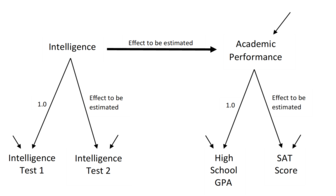
SEM involves a model representing how various aspects of some phenomenon are thought to causally connect to one another. Structural equation models often contain postulated causal connections among some latent variables (variables thought to exist but which can't be directly observed). Additional causal connections link those latent variables to observed variables whose values appear in a data set. The causal connections are represented using equations but the postulated structuring can also be presented using diagrams containing arrows as in Figures 1 and 2. The causal structures imply that specific patterns should appear among the values of the observed variables. This makes it possible to use the connections between the observed variables' values to estimate the magnitudes of the postulated effects, and to test whether or not the observed data are consistent with the requirements of the hypothesized causal structures.[5]
The boundary between what is and is not a structural equation model is not always clear but SE models often contain postulated causal connections among a set of latent variables (variables thought to exist but which can't be directly observed, like an attitude, intelligence or mental illness) and causal connections linking the postulated latent variables to variables that can be observed and whose values are available in some data set. Variations among the styles of latent causal connections, variations among the observed variables measuring the latent variables, and variations in the statistical estimation strategies result in the SEM toolkit including confirmatory factor analysis, confirmatory composite analysis, path analysis, multi-group modeling, longitudinal modeling, partial least squares path modeling, latent growth modeling and hierarchical or multilevel modeling.[6][7][8][9][10]
SEM researchers use computer programs to estimate the strength and sign of the coefficients corresponding to the modeled structural connections, for example the numbers connected to the arrows in Figure 1. Because a postulated model such as Figure 1 may not correspond to the worldly forces controlling the observed data measurements, the programs also provide model tests and diagnostic clues suggesting which indicators, or which model components, might introduce inconsistency between the model and observed data. Criticisms of SEM methods hint at: disregard of available model tests, problems in the model's specification, a tendency to accept models without considering external validity, and potential philosophical biases.[11]
A great advantage of SEM is that all of these measurements and tests occur simultaneously in one statistical estimation procedure, where all the model coefficients are calculated using all information from the observed variables. This means the estimates are more accurate than if a researcher were to calculate each part of the model separately.[12]
- ^ Cite error: The named reference
Salkind2007was invoked but never defined (see the help page). - ^ "Structural Equation Modeling". Encyclopedia of Epidemiology. 2008. doi:10.4135/9781412953948.n443. ISBN 978-1-4129-2816-8.
- ^ "Structural Equation Modeling". Encyclopedia of Educational Leadership and Administration. 2006. doi:10.4135/9781412939584.n544. ISBN 978-0-7619-3087-7.
- ^ "Structural Equation Modeling - an overview | ScienceDirect Topics". www.sciencedirect.com. Retrieved 2024-11-15.
- ^ Pearl, J. (2009). Causality: Models, Reasoning, and Inference. Second edition. New York: Cambridge University Press.
- ^ Kline, Rex B. (2016). Principles and practice of structural equation modeling (4th ed.). New York. ISBN 978-1-4625-2334-4. OCLC 934184322.
{{cite book}}: CS1 maint: location missing publisher (link) - ^ Hayduk, L. (1987) Structural Equation Modeling with LISREL: Essentials and Advances. Baltimore, Johns Hopkins University Press. ISBN 0-8018-3478-3
- ^ Bollen, Kenneth A. (1989). Structural equations with latent variables. New York: Wiley. ISBN 0-471-01171-1. OCLC 18834634.
- ^ Kaplan, David (2009). Structural equation modeling: foundations and extensions (2nd ed.). Los Angeles: SAGE. ISBN 978-1-4129-1624-0. OCLC 225852466.
- ^ Curran, Patrick J. (2003-10-01). "Have Multilevel Models Been Structural Equation Models All Along?". Multivariate Behavioral Research. 38 (4): 529–569. doi:10.1207/s15327906mbr3804_5. ISSN 0027-3171. PMID 26777445. S2CID 7384127.
- ^ Tarka, Piotr (2017). "An overview of structural equation modeling: Its beginnings, historical development, usefulness and controversies in the social sciences". Quality & Quantity. 52 (1): 313–54. doi:10.1007/s11135-017-0469-8. PMC 5794813. PMID 29416184.
- ^ MacCallum & Austin 2000, p. 209.